
Few months back, a HN post about learned indexes caught my attention. 83x less space with the same performance as a B-tree? What sort of magic trick is this?! And why isn’t everybody else using it if it’s so good?
I decided to spend some time reading the paper to really understand what’s going on. Now reading a scientific paper is a daunting endeavour as most of it is written in small text, decorated with magical Greek symbols, with little to no diagrams for us lay people. But this is really a beautiful piece of data structure which deserves to be used more widely in other systems, rather than just languish in academic circles.
So if you have been putting off from reading it, this post is my attempt at a simplified explanation of what is in the paper. No mathematical symbols. No equations. Just the basic idea of how it works.
What is an index
Let’s consider an array of sorted integers. We want to calculate the predecessor of x; i.e. given x, find out the largest integer in the array lesser than or equal to x. For example, if our array is {2,8,10,18,20}, predecessor(15) would be 10, and predecessor(20) would be 20. An extension of this would be the range(x, y) function, which would give us the set of integers lying within the range of x and y. Any data structure satisfying these requirements can be essentially considered as an index.
If we go through existing categories of data structures:
- Hash-based ones can only be used to “lookup” the position of a key.
- Bitmap-based indexes can be expensive to store, maintain and decompress.
- Trie-based indexes are mostly pointer based, and therefore take up space proportional to the data set.
Which brings us to B-tree based indexes and its variants being the go-to choice for such operations, and is widely used in all databases.
What is a learned index
In a learned index, the key idea is that indexes can be trained to “learn” this predecessor function. Naturally, the first thing that comes to mind is Machine Learning. And indeed, some implementation have used ML to learn this mapping of key to array position within an error approximation.
But unlike those, the PGM index is a fully dynamic, learned index, without any machine learning, that provides a maximum error tolerance and takes smaller space.
PGM Index
PGM means “piece-wise geometric model”. It attempts to create line segments that fit the key distribution in a cartesian plane. We call this a linear approximation. And it’s called “piece-wise” because a single line segment may not be able to express the entire set of keys, within a given error margin. Essentially, it’s a “piece-wise linear approximation” model. If all that sounds complicated, it really isn’t. Let’s take an example.
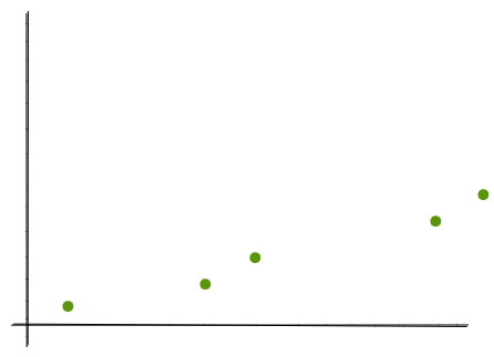
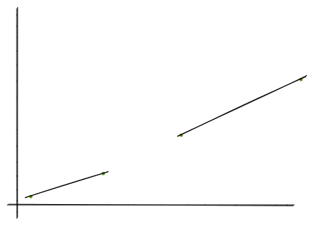
Consider the input data of {2,8,10,18,20} that we had earlier. Let’s plot these in a graph with the keys in the x-axis and array positions in the y-axis.
Now, we can see that we can express a set of points that are more or less linear, as a single line segment. Let’s draw a line for the points {2,0}, {8,1}, {10,2}.
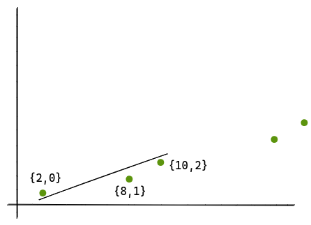
So any value lying within [2,10] can be mapped with this line. For example, let’s try to find predecessor(9). We take 9 to be the value of x and plot the value of y.
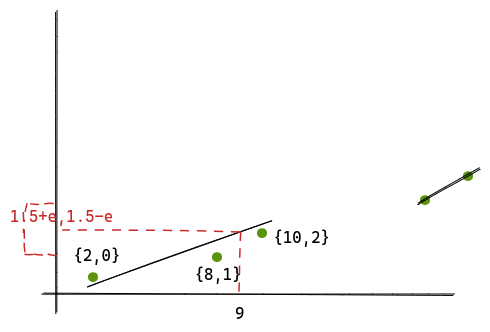
Once we get y, the algorithm guarantees that the actual value will lie within a range of {-e, +e}. And if we just do a binary search within a space of 2e + 1, we get our desired position.
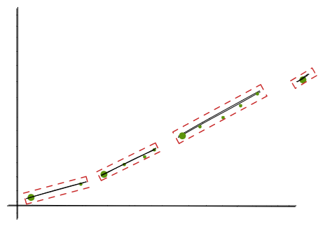
That’s all there is to it. Instead of storing the keys, we are just storing the slopes and intercepts, which is completely unrelated to the size of the data, but more dependent on the shape of it. The more random the data is, we need more line segments to express it. And on the other extreme, a set like {1,2,3,4} can be expressed with a single line with zero error.
But this leads to another problem. Once we have a set of line segments, each line segment only covers a portion of our entire key space. Given any random key, how do we know which line segment to use? It’s simple. We run the same algorithm again!
- Construction
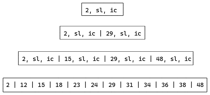
Let’s run through an example and see how do we build up the entire index. Assume our data set is {2, 12, 15, 18, 23, 24, 29, 31, 34, 36, 38, 48}. And error is e.
The algorithm to construct the index is as follows:
- We take each point from our set of
{k, pos(k)}, and incrementally construct a convex hull from those points. - At every iteration, we construct a bounding rectangle from the convex hull. This is a well-known computational geometry problem, of which there are several solutions. One of them is called Rotating Callipers.
- As long as the height of the bounding rectangle is not more than 2e, we keep adding points to the hull.
- When the height exceeds 2e, we stop our process, and construct a line segment joining the midpoints of the two arms of the rectangle.
- We store the first point in the set, the slope and intercept of the line segment, and repeat the whole process again.
At the end, we will get an array of tuples of (point, slope, intercept).
Now let’s wipe all the remaining points except the ones from the tuples and run the same algorithm again.
We see that each time, we get an array of decreasing size until we just have a root element. The in-memory representation becomes something like this:
- Search
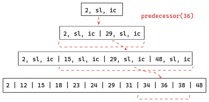
The algorithm to search for a value is as follows:
- We start with the root tuple of the index and compute the result of y =
k * sl + ic, for an input value ofk. - A lower bound
lois calculated to bey-eand a similar upper boundhiasy+e. - We search in the next array in
A[lo:hi]to find the rightmost element such thatA[i].key <= k - Once an element is found, the whole algorithm is repeated again to calculate
yof that node, and search in the next array. - This continues until we reach the original array, and we find our target position.
The paper proves that the number of tuples (m) for the last level will always be less than n/2e. Since this also holds true for the upper levels, it means that a PGM index cannot be worse than a 2e way B-tree. Because if at every level, we do a binary search within 2e +1, our worst case time complexity is O(log(m) + log(e)). However, in practice, a PGM index is seen to be much faster than a B-tree because m is usually far lower than n.
- Addition/Removal
Insertions and deletions in a PGM index are slightly tricker compared to traditional indexes. That is because a single tuple could index a variable and potentially large subset of data, which makes the classic B-tree node split and merge algorithms inapplicable. The paper proposes two approaches to handle updates, one customized for append-only data structures like time-series data. Another for general random update scenarios.
In an append-only scenario, the key is first added to the last tuple. If this does not exceeed e threshold, the process stops. If it does exceed, we create a new tuple with the key, and continue the process with the last tuple of the upper layer. This continues until we find a layer where adding the key remains within the threshold. If this continues till the root node, it gets split into two nodes, and a new root node gets created above that.
For inserts that happen in arbitrary positions, it gets slightly more complicated. In this case, we have to maintain multiple PGM indexes built over sets of keys. These sets are either empty or have size 20, 21 .. 2b where b = O(log(n)). Now each insert of a key k finds the first empty set, and builds a new PGM index from all the previous sets including the key k, and then the previous sets are emptied. Let’s take an example. Assume we are starting from scratch and we want to insert 3,8,1,6,9 in the index.
-
Since everything is empty, we find our first set S0 and insert 3. So our PGM looks like
S0 = [3] -
Now the next empty set is S1, because S0 is non-empty. So we take 3 from the last set, and add 8 to S1. S0 is emptied.
S0 = [] S1 = [3,8] -
Our next key is 1. The first empty set is S0. We just add 1 to S0 and move on.
S0 = [1] S1 = [3,8] -
Both S0 and S1 are non-empty now. So we move to S2, and empty S0 and S1.
S0 = [] S1 = [] S2 = [1,3,6,8] -
Again, the first empty set is S0. So 9 goes in it.
 S0 = [9]
 S1 = []
 S2 = [1,3,6,8]
The deletion of a key d is handled similar to an insert by adding a special tombstone value that indicates the logical removal of d.
Conclusion
And that was a very basic overview of the PGM index. There are further variants of this, fully described in detail in the paper. The successor from this is a Compressed PGM index which compresses the tuples. Then we have a Distribution-aware PGM index which adapts itself not only to the key distribution, but also to the distribution of queries. This is desirable in cases where it’s important to have more frequent queries respond faster than rare ones. Finally, we have a Multi-criteria PGM index that can be tuned to either optimize for time or optimize for space.
I have also created a port of the algorithm in Go here to understand the algorithm better. It’s just a prototype, and suffers from minor approximation issues. For a production-ready library, refer to the author’s C++ implementation here.
Lastly, I would like to thank Giorgio for taking the time to explain some aspects of the paper which I found hard to follow. His guidance has been a indispensable part in my understanding of the paper.
Links:
- Paper: http://www.vldb.org/pvldb/vol13/p1162-ferragina.pdf
- C++ implementation: https://github.com/gvinciguerra/PGM-index
- Website: https://pgm.di.unipi.it
